A Surprisingly Fast and Flexible Monte Carlo Option Pricer in Common Lisp
Recently, I’ve begun work on a dream project of mine: writing a quantative finance library in common lisp. After prodding the Claude LLM towards my vision, I unexpectedly ended up with a fast and flexible Monte Carlo options pricer which appears to outperform QuantLib’s C++ in speed and thread-invariance. Despite the library being far from complete, I nevertheless share what I think are promising signs, with a working example.
Monte Carlo Option Pricing with QuantLib
QuantLib is an open source quantitative finance library written in C++, and perhaps the most recognizable one among all quant libraries. To its credit, it is quite comprehensive, and correct. Unfortunately, it is a bit of a mess.
Since this article covers the specific task of pricing options with Monte Carlo methods, I will review the basics of what this task entails. An option is a financial contract that gives you the right (but not obligation) to purchase (or sell) a given financial asset at a certain agreed-upon price (a strike) on a set date (an expiry). Let’s focus on options that allow you to buy shares of a stock—a call option. How should we price this contract?
To answer this, let’s address a toy example. I offer to play a game with you
where I roll a fair 6-sided die and pay you the amount of the face it lands on.
What should I set the cost of admission to this game? Being the “house”, I
certainly don’t want to lose money, so amounts like $1 probably don’t make sense
for me. On the other hand, values like a $6 admission fee won’t give the players
of the game any winnings. Where is the happy medium?
If I expect to drive large demand to play this game, I should price the admission no less than what an average roll of a 6-sided die to be. The average in this case is the expected value of single roll of a die. The exact value of this is 3.5. Obviously, you can never roll a 3.5 on a die, but pricing the admission in this way ensures that—assuming high demand for the game—I won’t lose money. Let’s model the average payout over 100, 1000, and 10000 games of this type. Notice that the more games we play, the closer we get to 3.5.
(defun roll-die ()
  "Return a random integer from 1 through 6."
  (1+ (random 6)))

(defun average-roll (rolls)
  "Simulate ROLLS throws and return their average."
  (/ (loop repeat rolls
           sum (roll-die))
     (float rolls)))

(let ((*random-state* (make-random-state t)))
  (format t "Theoretical expected value: 3.5~%")
  (dolist (rolls '(100 1000 10000 100000))
    (format t "~4D rolls: average = ~,3F~%"
            rolls
            (average-roll rolls))))
Theoretical expected value: 3.5
 100 rolls: average = 3.710
1000 rolls: average = 3.519
10000 rolls: average = 3.506
100000 rolls: average = 3.510
Pricing equity options is no different: the fair price of the option should be the value you expect to receive from owning the equity at the agreed-upon price (discounted by the risk-free rate, but let’s ignore that for now). If \(S_T\) is the value of the equity at the time of exercise, and \(K\) is the price you agreed to buy it at, the immediate payoff of the option \(\max (S_T - K, 0)\), where the \(0\) payoff comes from not exercising the right to buy because \(S_T < K\) (we assume you are rational and wouldn’t willingly overpay for the equity).
So what is the expected payoff of the option? This is where things get significantly complicated. Using our fair die example, we can approximate the value \(S_T\) of a stock at exercise time, and average over all of these endpoints. But to simulate the expected value of an equity at time of exercise, you’d need to know how the equity moves before the fact. If you could successfully do this even half of the time, you would not be reading this and would be fabulously wealthy. Hence, we need to pick a model that describes the dynamics of our equity in the future (called a stochastic process).
Once a model is chosen, you can price a call option. Just simulate \(N\) equity paths with your process, and compute the average of \(\max (S_T-K,0)\) for each predicted value of the equity at the exercise/expiry time, and that’s your option value. The larger your \(N\), the closer you will get to the actual fair value of the option with your assumed asset’s underlying dynamics.
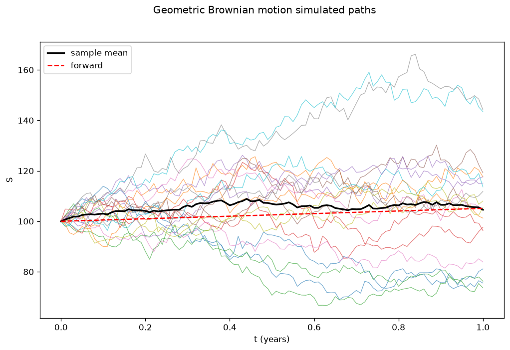
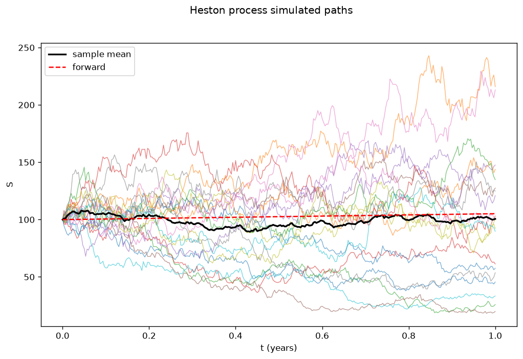
Here are some possible equity paths simulated by two different models: geometric Brownian motion, and the Heston process. The specifics of how these models are constructed are far beyond the scope of this article. The bottom line is that all you need to price an option (or any instrument that pays based on the final value of some stochastic process) is a model for your underlying asset, and a way to step forward in time with this model.
Pricing Options in QuantLib
How does the process of pricing options look in QuantLib? Unfortunately, it depends heavily on the model you choose. The general workflow after choosing a model for equity prices is as follows:
[ StochasticProcess ] ──> [ PathGenerator ] ──> [ PathPricer ] ──> [ MCVanillaEngine ]
(Model Definition)        (Step forward in time) (Evaluate payoff    (Averages & PV)
                                                  at path ends)
An example of pricing of pricing an option whose underlying stock follows the variance gamma process is given.
QuantLib Variance Gamma option pricing example
#include <ql/quantlib.hpp>
#include <iostream>

using namespace QuantLib;

int main() {
    Calendar calendar = TARGET();
    Date today = Date::todaysDate();
    Settings::instance().evaluationDate() = today;

    DayCounter dc = Actual365Fixed();
    Date maturity = today + Period(1, Years);
    Time T = dc.yearFraction(today, maturity);

    Real s0 = 100.0;
    Rate r = 0.05;
    Rate q = 0.02;

    Handle<Quote> spot(ext::make_shared<SimpleQuote>(s0));
    Handle<YieldTermStructure> riskFreeRate(
        ext::make_shared<FlatForward>(today, r, dc));
    Handle<YieldTermStructure> dividendYield(
        ext::make_shared<FlatForward>(today, q, dc));

    auto process = ext::make_shared<VarianceGammaProcess>(
        spot, dividendYield, riskFreeRate, 0.20, 0.15, -0.10);

    TimeGrid grid(T, 1);

    PathGenerator<PseudoRandom::rsg_type> pathGen(
        process, grid, PseudoRandom::make_sequence_generator(grid.size() - 1, 42), false);

    PlainVanillaPayoff payoff(Option::Call, 100);
    DiscountFactor df = riskFreeRate->discount(T);

    Accumulator priceAccumulator;

    for (Size i = 0; i < 100000; ++i) {
        const Path& path = pathGen.next().value;
        Real terminalPrice = path.back(); // ST

        Real payoffValue = payoff(terminalPrice);
        priceAccumulator.add(payoffValue);
    }

    Real mcPrice = priceAccumulator.mean() * df;
    Real standardError = priceAccumulator.errorEstimate() * df;

    std::cout << "MC Price: " << mcPrice
              << " +/- " << standardError << std::endl;

    return 0;
}
Once you get over the zoo of classes involved to do such a basic operation, it’s a straightforward piece of code. It turns out that on some assumed equity processes like the Heston model from above, the library provides explicit classes to make Monte Carlo pricing more terse:
int main() {
    Calendar calendar = TARGET();
    Date today = Date::todaysDate();
    Settings::instance().evaluationDate() = today;

    DayCounter dc = Actual365Fixed();
    Date maturity = today + Period(1, Years);

    // Option and market data
    Real s0 = 100.0;
    Real strike = 100.0;
    Rate r = 0.05;
    Rate q = 0.02;

    //  Model Parameters
    Real v0    = 0.04;  // Initial variance (vol = 20%)
    Real kappa = 2.0;   // Mean reversion speed
    Real theta = 0.04;  // Long-term variance
    Real sigma = 0.30;  // Volatility of variance
    Real rho   = -0.70; // Asset-variance correlation

    // Handles and Process Setup
    Handle<Quote> spot(ext::make_shared<SimpleQuote>(s0));
    Handle<YieldTermStructure> riskFreeRate(
        ext::make_shared<FlatForward>(today, r, dc));
    Handle<YieldTermStructure> dividendYield(
        ext::make_shared<FlatForward>(today, q, dc));

    auto process = ext::make_shared<HestonProcess>(
        riskFreeRate, dividendYield, spot, v0, kappa, theta, sigma, rho);

    auto payoff = ext::make_shared<PlainVanillaPayoff>(Option::Call, strike);
    auto exercise = ext::make_shared<EuropeanExercise>(maturity);
    EuropeanOption option(payoff, exercise);

    // Simulation parameters
    Size timeSteps = 100;    // Time grid resolution for Euler discretization
    Size nSamples  = 50000;  // Total simulated paths
    BigNatural seed = 42;

    auto engine = ext::make_shared<MCHestonEuropeanEngine<LowDiscrepancy>>(
        process,
        timeSteps,
        Null<Size>(),      // stepsPerYear (optional if timeSteps is specified)
        false,             // brownianBridge
        false,             // antitheticVariates
        nSamples,          // requiredSamples
        Null<Real>(),      // requiredTolerance
        nSamples,          // maxSamples
        seed               // seed
    );

    option.setPricingEngine(engine);

    std::cout << "MCHestonEuropeanEngine Price: " << option.NPV() << std::endl;
    std::cout << "Engine Error Estimate:       " << option.errorEstimate() << std::endl;

    return 0;
}
There are 19 factory classes in QuantLib defining Monte Carlo engines, a couple
of which are relevant to pricing our European option (MakeMCEuropeanHestonEngine
and MakeMCEuropeanGJGARCHEngine). QuantLib leaves it up to the user to glue all
of the classes to price an option together. Mathematically, however, all you
need is a process to model your underlying asset and formula for how your option
payoff looks. Can this be made any easier?
Monte Carlo Option Pricing with fincl
Fincl adopts the same core assumptions as QuantLib: to price an option, you need an option, a market to price within, and an engine to price it with. Since we’ve already fixed the other variables, let’s discuss how fincl handles the Monte Carlo engine differently.
Since extensibility of the library itself was of major importance, the friction of defining your own stochastic process (a toy or otherwise) and pricing an option with it should be as minimal as possible. By specializing a generic function on stochastic processes that step forward in time, we can simultaneously tame the combinatorial explosion of classes seen in QuantLib and make a single, high-level entry point into simulating the process.
This choice presented a slight issue: multiple dispatch in CLOS is slow. Calling
generics possibly hundreds of thousands of times in a Monte Carlo simulation was
undesirable. This problem is actually present in QuantLib in different clothing,
the stepper class calls virtual functions drift() and diffusion(), which comes
back to bite when speed is scrutinized. To solve this in fincl, the generic
should instead return a lambda editing the state of the process in-place so that
a Monte Carlo simulation with this stepper can dispatch on this function exactly
once.
A Toy Option Contract
Let me illustrate the extensibility of fincl while showing how this “return a lambda” business works. We can use it to determine the price of an option on our die game from before. Say that a call option on the game gives you the right (but not obligation) to buy into the die game for a agreed-upon fee after the die has been rolled. What is the price of this option? From before, the option is fairly priced at the value you’d expect to earn from holding and exercising this contract.
For example, suppose you want to buy an option that allows you to enter the game
at an admission price of $2. I roll the die, and you observe the outcome. Under
which conditions would you exercise this option? Obviously, you want to make
money, so you’d only buy into the game at $2 if the die rolls one of 3,4,5,6,
and you exercise the option. If the die rolls 1 or 2, you are at best
indifferent and do not exercise. What is the expected payout of buying into the
game at $2? In each of the cases where you exercise, you earn $1, $2, $3, and
$4, respectively. The expected profit is the sum of these payouts weighted by
the probability that they occur, all of which are an equal \(\frac{1}{6}\). The
expected payoff is
\[\mathbb{E}[\max( X - 2 , 0 )] = \frac{1+2+3+4}{6}\approx 1.667.\]
The fair price of this option is around $1.667. Let’s model it in fincl.
fincl offers macros to easily define stochastic processes with minimal code repetition. As mentioned before, we need to define the process, an initial state, and a stepper which returns a lambda that steps forward in time.
Setup for fincl
(defpackage #:die-game
  (:use #:cl #:fincl))

(in-package #:die-game)
;; For date and tenor literals
(named-readtables:in-readtable fincl:syntax)

;; Not actually needed, the fair dice is not
;; dependent on time
(defconstant +today+ #D"2026-10-01")
We can make fincl aware of our die roll process and define how it steps in time.
(define-process fair-die (stochastic-process) (:state-size 1)
                ()
                (:documentation "Rolling a fair die. State is the previous
roll."))

(defmethod initial-state ((p fair-die) market)
  (declare (ignore market))
  (make-array 1 :element-type 'double-float
                :initial-element 0d0))

(defmethod make-stepper ((p fair-die) market times)
  (declare (ignore market times))
  ;; STATE is a size 1 array containing the most recent roll
  ;; NORMALS is a size 1 array containing a standard normal
  ;; J is the time index on a path (irrelevant here)
  (lambda (state normals j)
    (declare (ignore j))
    ;; Convert standard normal to discrete U(1,6)
    (let ((roll (+ 1d0 (min 5d0 (ffloor (* 6d0 (norm-cdf (aref normals 0))))))))
      ;; Update current game's roll
      (setf (aref state 0) roll))
    nil))
With the dynamics of our game settled, we can declare our contract and the market it will be priced in.
;; right to buy into the game, struck at $2 admission fee
(defparameter *die-contract* (make-option (call 2)
                                          (expires #T"1Y" :from +today+)))

(defparameter *market* (make-bs-market :valuation-date +today+
                                       ;; Spot and vol ignored
                                       :spot 1
                                       :vol 1
                                       ;; Rate 0, otherwise used for discounting
                                       :rate 0))
With the ingredients to price all accounted for, we can hand our stochastic process (our fair die) over to the Monte Carlo engine and price our option contract:
(defparameter *mc-engine* (make-engine :mc :process (make-fair-die)
                                           :n-paths 1000000
                                           :n-steps 1))

(multiple-value-bind (npv se engine) (price *die-contract* *mc-engine* *market*)
  (format t "~&price ~,4F~%standard error: ~,4F~%(~A)~%" npv se engine))
price 1.6667
standard error: 0.0003
(#<ENGINE (make-engine :mc :process (die-game::make-fair-die) :n-paths 1000000
                       :n-steps 1)>)
We choose 1 step per simulation path since the uniform die roll does not depend on time. We can also play around with the option and observe that the other strike prices (hint, we should expect to pay more for an option as we strike a lower entry fee, since there are more exercise conditions.) Using simulations, we have recovered our theoretical fair price for our die game option!
Bonus for experts or the curious
If we suppose the terms of an American *die-contract* option allow you to buy
into the game after any of the next 100 rolls, we can price this with fincl as well:
(defparameter *american-die-call*
         (make-option (american) (call 2) (expires #T"1Y" :from +today+)))
(defparameter *mc-engine* (make-engine :mc :process (make-fair-die)
                                           :n-paths 10000
                                           :n-steps 100))
(price *american-die-call* *mc-engine* *market*)
;;; => 4.0d0
;;;    0.0d0
;;;    #<ENGINE (make-engine :mc :process (die-game::make-fair-die) :n-paths 10000
;;;                      :n-steps 100)>
Are there scenarios where we make money exercising this contract? The obviously
optimal exercise time is as soon as I roll a 6, Assuming I roll a 6 in the next
100 rolls, you get paid \(\$6-\$2 = \$4\), leaving you with net zero change in
cash.
This reflects the fact that a 6 will appear in 100 rolls with near certainty (I
can roll zero sixes in 100 rolls with probability \(1.22 \times 10^{-8}\)), so
you can always hold out for an exercise time with maximum payoff.
Performance
What surprised me about this architecture choice in fincl was the performance. Across all option pricing jobs that I’ve benchmarked, fincl appears to beat the equivalent QuantLib in single-threaded tasks on my machine. The gap only grows when you consider multiple workers, which QuantLib cannot do natively.
On average, fincl outperforms QuantLib by a factor of 4, with the gap widening with more workers. Precision is a mixed bag; against (semi)analytically derived reference option prices, fincl is anywhere between 3 times and 1/10th more precise (absolute difference).
Benchmarked Monte Carlo test results with miscellaneous notes on architectural differences
== monte-carlo (1 worker; extra rows at 4) =======================================
 benchmark                 QuantLib value        fincl value  diff (se)  verdict  QuantLib median [min] ±MAD  fincl median [min] ±MAD  ratio  per path (QL / fincl)  per step (QL / fincl)  cost to 1e-3 se (QL / fincl)  fincl consed  QL setup  fincl setup
 mc-european-gbm          9.20916 ± 0.033    9.20069 ± 0.032     -0.18σ    agree       95.3 ms [95.0 ms] ±0%    15.1 ms [14.9 ms] ±1%  0.16x        953 ns / 151 ns        953 ns / 151 ns                101 s / 15.9 s        4.3 MB   89.5 us      3.09 ms
   [fincl, 4 workers]                        9.20069 ± 0.032                                                    7.91 ms [6.24 ms] ±4%  0.08x           -- / 79.1 ns           -- / 79.1 ns                   -- / 8.35 s        4.3 MB                 160 us
 mc-european-gbm-sobol          9.2261448  9.22843 ± 8.7e-04      2.61σ    agree         105 ms [104 ms] ±0%    48.7 ms [45.5 ms] ±5%  0.46x       1.05 us / 487 ns       1.05 us / 487 ns                  -- / 37.2 ms       29.3 MB   23.5 us       229 us
   [fincl, 4 workers]                      9.22843 ± 8.7e-04                                                   25.2 ms [19.0 ms] ±13%  0.24x            -- / 252 ns            -- / 252 ns                  -- / 19.2 ms       29.4 MB                 166 us
 mc-european-heston       9.10751 ± 0.023    9.07744 ± 0.023     -0.92σ    agree         6.23 s [6.23 s] ±0%      1.99 s [1.97 s] ±1%  0.32x      62.3 us / 19.9 us       1.25 us / 398 ns               3321 s / 1044 s     1300.9 MB   23.3 us       368 us
   [fincl, 4 workers]                        9.07744 ± 0.023                                                      838 ms [795 ms] ±1%  0.13x           -- / 8.38 us            -- / 168 ns                    -- / 440 s     1302.9 MB                2.49 ms
 mc-asian-arith-cv      5.51423 ± 8.6e-04  5.51302 ± 7.0e-04     -1.09σ    agree         1.06 s [1.06 s] ±0%      305 ms [297 ms] ±1%  0.29x      10.6 us / 3.05 us        886 ns / 254 ns               792 ms / 150 ms      121.2 MB   27.1 us       310 us
   [fincl, 4 workers]                      5.51302 ± 7.0e-04                                                      142 ms [125 ms] ±3%  0.13x           -- / 1.42 us            -- / 118 ns                  -- / 69.6 ms      121.5 MB                 204 us
 mc-barrier-down-out      7.60312 ± 0.036    7.63285 ± 0.036      0.59σ    agree         24.9 s [24.9 s] ±0%      3.51 s [3.50 s] ±0%  0.14x       249 us / 35.1 us        987 ns / 139 ns              31613 s / 4487 s        2.6 MB   26.2 us       315 us
   [fincl, 4 workers]                        7.63285 ± 0.036                                                      1.32 s [1.11 s] ±0%  0.05x           -- / 13.2 us           -- / 52.2 ns                   -- / 1682 s        2.6 MB                 180 us
 mc-american-lsm          6.65484 ± 0.014    6.65759 ± 0.014      0.14σ    agree         10.7 s [10.7 s] ±0%      2.43 s [2.40 s] ±0%  0.23x       107 us / 24.3 us       2.15 us / 485 ns                2112 s / 491 s      420.4 MB   18.5 us       482 us
   [fincl, 4 workers]                        6.65759 ± 0.014                                                      1.11 s [1.10 s] ±0%  0.10x           -- / 11.1 us            -- / 223 ns                    -- / 225 s      421.3 MB                 226 us

 geometric mean of the ratios: 0.24x (fincl faster); 0 DIFFER, 0 without QuantLib, 0 ERROR
   mc-european-gbm against the reference 9.2270055: QuantLib -0.018, fincl -0.026
 mc-european-gbm-sobol: QuantLib's Sobol estimate has no valid standard error (its sample standard deviation ignores the low discrepancy), so the verdict uses fincl's, from 16 randomizations; neither side uses antithetics
   mc-european-gbm-sobol against the reference 9.2270055: QuantLib -8.6e-4, fincl 1.4e-3
 mc-european-heston: both use Andersen's quadratic-exponential scheme with the martingale correction
   mc-european-heston against the reference 9.0595069: QuantLib 0.048, fincl 0.018
 mc-asian-arith-cv: QuantLib corrects with a fixed coefficient of 1 on the geometric Asian, fincl with the regression coefficient
 mc-barrier-down-out: QuantLib samples the crossing with a uniform per step, fincl weights by the survival probability
   mc-barrier-down-out against the reference 7.5869540: QuantLib 0.016, fincl 0.046
 mc-american-lsm: both fit the exercise rule on one path set and price on another (fincl :lsm-valuation :independent), a low-biased estimate of the 50-date Bermudan
   mc-american-lsm against the reference 6.6606893: QuantLib -5.8e-3, fincl -3.1e-3
Equating the two libraries for speed, it’s not hard to believe that fincl could achieve the same precision in equal or less time. It’s important to keep in mind that in the real world, Monte Carlo is actually a last resort. Complex exotic option types that have no closed form formulas, even under unrealistic assumptions about how the underlying asset moves, sometimes have no approximations in closed form. This is the only situation where reaching for Monte Carlo is the first course of action.
Despite this, I believe that any quant finance library worth its salt should have solid support for MC simulations. In the end, it is the most general of all options pricing methods, and is agnostic to choice of process.I’m glad one exists in common lisp now.